Dynamic panels · Other

Arellano-Bond Estimation for Dynamic Panels

Arellano-Bond uses lagged levels as instruments after differencing away unit effects.

Why fixed effects are difficult with lagged outcomes

Consider

$$ y_{it}=\rho y_{i,t-1}+\beta x_{it}+\alpha_i+u_{it}. $$

First differencing removes $\alpha_i$:

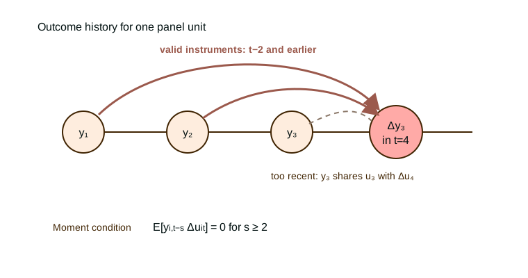
$$ \Delta y_{it}=\rho\Delta y_{i,t-1}+\beta\Delta x_{it}+\Delta u_{it}. $$

The differenced lag remains correlated with $\Delta u_{it}$. Deeper lagged levels provide instruments when level errors have no serial correlation and past outcomes are orthogonal to future innovations (Arellano and Bond, 1991).

$$ E[y_{i,t-s}\Delta u_{it}]=0,\qquad s\ge2. $$

A triangular instrument matrix

For five dates, the available outcome instruments expand over time.

Differenced equation	Available level instruments
$t=3$	$y_1$
$t=4$	$y_1,y_2$
$t=5$	$y_1,y_2,y_3$

This triangular structure is the central visual for difference GMM.

Timeline showing that levels dated t minus 2 and earlier can instrument the differenced lagged outcome at time t. — Instrument timing after first differencing. Earlier outcome levels can instrument the endogenous change in the lagged outcome.

Assumptions and implementation

The moment conditions require restrictions on serial correlation and regressor timing. Difference GMM can have weak instruments when outcomes are persistent. Instrument proliferation can overfit endogenous variables and weaken specification tests.

One-step, two-step, difference, system, collapsed, and uncollapsed specifications define different estimators. Two-step standard errors need finite-sample correction (Windmeijer, 2005).

Interpreting the dynamic coefficient

The coefficient on $y_{i,t-1}$ describes persistence after the included covariates and unit effects are controlled. When its magnitude is below one, a one-unit innovation has effects that decay over later periods. The short-run coefficient on $x_{it}$ differs from its long-run effect. Under a stable linear model, the latter is $\beta/(1-\rho)$, where $\rho$ is the lagged-outcome coefficient.

This interpretation relies on valid lag instruments. The triangular matrix in the figure shows that earlier levels enter only when timing makes them orthogonal to the differenced error. More periods create more possible instruments, which can become a problem.

Moment checks and instrument discipline

Sort observations by unit and time before creating differences and lags. Report whether the panel is balanced and how gaps are handled. Specify the first and last instrument lags for each endogenous, predetermined, and exogenous variable. Keep the instrument count well below the number of units when possible. Collapsing the matrix or restricting lag depth reduces proliferation.

First-differenced errors should show first-order serial correlation. They should not show second-order serial correlation under the standard moment conditions. Report both tests. Also report the Hansen or Sargan statistic with its instrument count. A high Hansen value can reflect weak tests from too many instruments, so it is not automatic evidence of validity. Compare parsimonious instrument sets and inspect coefficient stability. Two-step estimates need the Windmeijer finite-sample covariance correction. (Arellano and Bond, 1991)

Source status

Arellano and Bond 1991 and Nickell 1981 remain manual-access sources in the local audit.

Sources and further reading

Manuel Arellano, Stephen Bond. 1991. “Some Tests of Specification for Panel Data: Monte Carlo Evidence and an Application to Employment Equations.” Review of Economic Studies 58(2): 277--297. doi:10.2307/2297968.
Frank Windmeijer. 2005. “A Finite Sample Correction for the Variance of Linear Efficient Two-Step GMM Estimators.” Journal of Econometrics 126(1): 25--51. doi:10.1016/j.jeconom.2004.02.005.
David Roodman. 2009. “How to Do xtabond2: An Introduction to Difference and System GMM in Stata.” Stata Journal 9(1): 86--136. doi:10.1177/1536867X0900900106.

About this benchmark task

Status: In the benchmark
Identifier: dynpanel_ab
Family: Other
Software: Stata, R, Python
Source: Benchmark task set

Task statement

Estimate the one-step Arellano-Bond difference GMM dynamic panel model for y on its first lag and x (equivalent to Stata `xtabond y x, lags(1)` or R `plm::pgmm(y ~ lag(y, 1) + x | lag(y, 2:99), effect = "individual", model = "onestep", transformation = "d")`): first-difference the equation, use GMM-type instruments (all available lags of y from t-2 and earlier, one instrument column per lag and period; do not collapse the instrument matrix) for the lagged dependent variable, and use x in first differences as a standard instrument. Use the standard one-step weighting matrix built from the first-difference operator. Do not use two-step GMM, system GMM, or time dummies. Report coefficient rows rho for the lagged dependent variable and beta_x for x. Standard errors are not part of this benchmark task; set se to null for both rows.

Required output

rho, beta_x

Open every recorded run for this task.