Time series

Local-projection impulse response

Local projections estimate one regression for each response horizon.

The task

Task statement

Estimate the local projection y_{t+4} on shock_t and y_{t-1}, with an intercept, using Newey-West standard error with lag 4. Report row irf_h4.

Data

Columns: t, y, shock.

Files: input.csv

Required output

Scored estimates: irf_h4.

The standard errors of irf_h4 are also scored, because the main decision in this task is how to compute them.

Reference output

Term	Reference estimate	Reference standard error	Sample size
`irf_h4`	0.11267202	0.083956171	245

A run succeeds when every scored estimate lies within 1 percent or 0.005 of its reference value, whichever is larger, and every scored standard error lies within 1 percent of the reference or of an accepted alternative convention. Sample sizes are not scored.

Task success

Agency condition	Claude Sonnet 4.6	GPT-5.6 Luna
Chatbot	78.3%	81.7%
Self-repair	98.3%	98.3%
Constrained agent	100.0%	98.3%

All runs: 92.5% of 360 runs
By prompt condition: Zero-shot 97.2%, One-shot 87.8%
By software: Python 100.0%, R 94.2%, Stata 83.3%

One equation per horizon

Local projections estimate the response at horizon $h$ directly (Jorda, 2005).

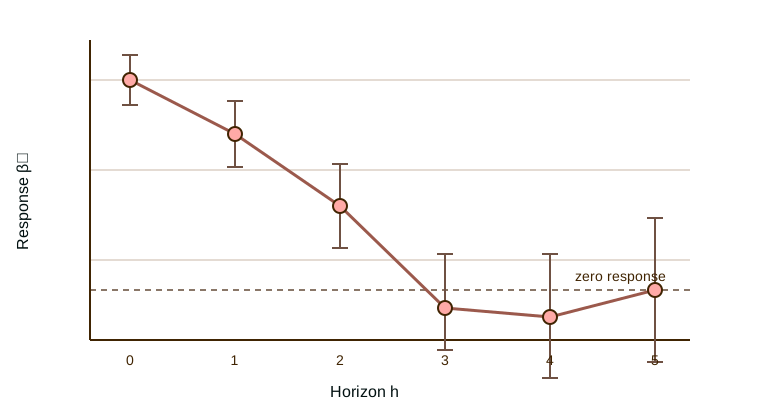
$$ y_{t+h}=\alpha_h+\beta_h shock_t+\Gamma_h'W_t+u_{t+h}. $$

The sequence $\{\beta_h\}$ is the impulse response. Each horizon can use the same controls and a separate covariance estimate.

A four-horizon response

Horizon $h$	$\hat\beta_h$	Interpretation
0	1.00	Impact response
1	0.70	One period later
2	0.30	Two periods later
3	-0.10	Mild reversal

The cumulative response through horizon three is $1.00+0.70+0.30-0.10=1.90$.

Local-projection impulse response estimates with uncertainty intervals across horizons zero through five. — Each point comes from a separate horizon regression. Vertical intervals show horizon-specific uncertainty.

Assumptions and implementation

Shock identification and control selection determine the causal interpretation. Serial correlation and overlapping outcomes create horizon-dependent error dependence.

Newey-West inference requires a kernel, a lag length, and a finite-sample convention. Software can also shift lead and lag indexing. The horizon-flow figure tracks one shock through separate outcome equations.

Reading the response path

Each local-projection coefficient answers a separate horizon question. If $x_t$ is a one-unit innovation, $\beta_h$ is the expected change in $y_{t+h}$ associated with that innovation after the stated controls. Plot the estimates against $h$ with confidence bands and a zero line. State whether the response is in levels, growth rates, or cumulative units.

A cumulative response through horizon $H$ is a sum of horizon-specific effects only when the equations and outcome transformation support that definition. Its standard error must include covariance across estimates. Pointwise bands describe each horizon separately. Simultaneous bands address coverage of the full plotted path.

Specification and uncertainty

Use a common sample across horizons when direct curve comparisons require it. Otherwise, report the changing observation count. Select lags before viewing the preferred response and keep the control set consistent with the shock identification. Forecast overlap induces serial correlation in horizon residuals, especially for $h>0$. Use a covariance estimator or bootstrap that reflects this dependence and any panel clustering.

Local projections are flexible, but long horizons can be noisy because fewer effective observations remain. Inspect sensitivity to lag length, trend terms, horizon range, and extreme shocks. If $x_t$ is not externally identified, the curve describes a conditional association. Recursive, proxy, or narrative identification adds assumptions that must be stated. Label the shock normalization because a one-standard-deviation and one-unit response have different scales. (Jorda, 2005)

Sources and further reading

Oscar Jorda. 2005. “Estimation and Inference of Impulse Responses by Local Projections.” American Economic Review 95(1): 161–182. doi:10.1257/0002828053828518.
Mikkel Plagborg-Moller, Christian K. Wolf. 2021. “Local Projections and VARs Estimate the Same Impulse Responses.” Econometrica 89(2): 955–980. doi:10.3982/ECTA17813.

About this benchmark task

Method group: Time series
Software: Stata, R, and Python
Runs: 360 runs, ten in each combination of model, software, prompt, and agency condition

Open every recorded run for this task.