Causal inference · Regression discontinuity
Sharp Regression Discontinuity
A sharp regression-discontinuity design identifies a local treatment effect from a jump at a known cutoff.
A discontinuity in treatment assignment
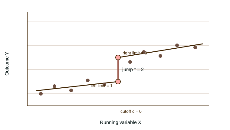
In a sharp design, treatment switches from zero to one at cutoff $c$. The target is the difference between the two conditional-mean limits (Imbens and Lemieux, 2008).
A local example
Suppose local linear fits near zero are
| Side | Intercept at zero | Local slope |
|---|---|---|
| Left | 1 | 0.5 |
| Right | 3 | 0.2 |
The estimated jump is $3-1=2$.
Assumptions
Potential-outcome conditional means must be continuous at the cutoff. Units must not sort precisely around the threshold in a way that creates other jumps. The estimate is local to the cutoff.
Estimation choices
Local polynomial order, kernel, bandwidth, bias correction, and covariance estimator all affect reported output. A narrow bandwidth reduces approximation bias and uses less information. Modern robust bias correction adjusts both the estimate and its uncertainty (Calonico et al., 2014).
The page figure places separate local fits on both sides of the cutoff and labels their boundary jump.
Interpretation and reporting
The estimated treatment jump is the right intercept minus the left intercept. In the example, the result is $3-1=2$. The two slopes describe nearby outcome trends and do not change that boundary subtraction.
Report the cutoff, bandwidth, kernel, polynomial order, side-specific sample counts, and bias correction. Place the figure beside the numerical estimate. The graph should reveal whether observations support both fitted limits near zero.
This effect applies to units at the threshold. It should not be read as an average effect for the full sample. Manipulation, another policy at the same cutoff, or a discontinuous composition change can undermine identification.
Reproducible implementation
Center the running variable so the cutoff equals zero. Construct treatment from the deterministic assignment rule. Restrict observations to the chosen bandwidth and apply the declared kernel weights.
Fit side-specific local polynomials or an equivalent interacted regression. Evaluate both fits at zero and subtract their intercepts. Use the matching robust bias-corrected procedure for uncertainty.
Check density around the cutoff (McCrary, 2008) and plot predetermined covariates. Repeat the analysis with nearby bandwidths and inspect sensitivity to high-weight boundary observations. Save binned-plot settings separately from estimation settings because visual bins do not define the estimator (Calonico et al., 2014).
Further reading
Imbens and Lemieux give a practical guide to RD analysis (Imbens and Lemieux, 2008). Calonico, Cattaneo, and Titiunik develop robust bias-corrected inference (Calonico et al., 2014).
Source status
- Hahn, Todd, and Van der Klaauw 2001 remains a source gap in the local task folder.
Sources and further reading
- Guido W. Imbens, Thomas Lemieux. 2008. “Regression Discontinuity Designs: A Guide to Practice.” Journal of Econometrics 142(2): 615--635. doi:10.1016/j.jeconom.2007.05.001.
- Sebastian Calonico, Matias D. Cattaneo, Rocio Titiunik. 2014. “Robust Nonparametric Confidence Intervals for Regression-Discontinuity Designs.” Econometrica 82(6): 2295--2326. doi:10.3982/ECTA11757.
- Justin McCrary. 2008. “Manipulation of the Running Variable in the Regression Discontinuity Design: A Density Test.” Journal of Econometrics 142(2): 698--714. doi:10.1016/j.jeconom.2007.05.005.
About this benchmark task
- Status
- In the benchmark
- Identifier
rdd_sharp- Family
- Regression discontinuity
- Software
- Stata, R, Python
- Source
- Benchmark task set
Task statement
Using bandwidth h = 0.5 and triangular kernel weights, fit local linear regressions on each side of cutoff z = 0 and report the difference in intercepts as row late.
Required output
late