Causal inference · Difference-in-differences
Difference-in-Differences with Staggered Treatment Timing
Group-time treatment effects separate cohorts and dates when treatment begins at different times.
Staggered difference-in-differences applies when units start treatment on different dates. Schools can adopt a program in different years. States can enact a law in different quarters. Each adoption date defines a treatment cohort.
The cohort-time object
Let $G_i=g$ mean that unit $i$ first receives treatment in period $g$. Let $G_i=\infty$ identify units that never receive treatment. The central estimand is the average treatment effect for cohort $g$ in period $t$ (Callaway and Sant'Anna, 2021).
This notation keeps two sources of variation visible. Effects can differ across cohorts. They can also change with exposure length $e=t-g$. A single pooled coefficient hides both dimensions.
Reading the adoption matrix
Consider three cohorts and a never-treated group. The letters U and T mark untreated and treated observations.
| Group | Period 1 | Period 2 | Period 3 | Period 4 |
|---|---|---|---|---|
| $G=2$ | U | T | T | T |
| $G=3$ | U | U | T | T |
| $G=4$ | U | U | U | T |
| $G=\infty$ | U | U | U | U |
For $ATT(3,4)$, cohort 3 has one untreated base period and two treated periods. The never-treated row supplies an untreated comparison at period 4. A not-yet-treated comparison can also use cohort 4 before its adoption.
The matrix shows which comparisons are available. It also shows why an already-treated cohort cannot represent an untreated outcome.
Identification with a comparison group
Suppose period $g-1$ is the base period. Under no anticipation and parallel trends with never-treated units,
No anticipation means treatment does not change outcomes before adoption. Parallel trends means untreated outcomes would have changed equally for both groups. This assumption concerns the untreated potential outcome. It does not require equal outcome levels.
Covariate adjustment replaces unconditional parallel trends with a conditional version. The covariates must be measured before treatment when treatment can affect them.
A numerical group-time effect
Suppose cohort 3 has a mean outcome of 10 in period 2 and 15 in period 4. Never-treated units move from 8 to 10.
| Group | Base mean | Period 4 mean | Change |
|---|---|---|---|
| Cohort 3 | 10 | 15 | 5 |
| Never treated | 8 | 10 | 2 |
The estimate is
The value 3 is specific to cohort 3 and period 4. It need not equal $ATT(2,4)$ or $ATT(3,3)$.
From group-time effects to summaries
An overall effect combines identified cells with declared weights.
Cohort weights answer an adoption-cohort question. Calendar weights answer a date-specific question. Event-time weights summarize effects after $e$ periods of exposure. The reported label should name the aggregation.
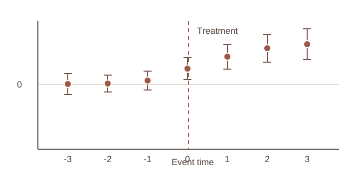
An event-study graph plots estimates against $e=t-g$. Pre-treatment points can reveal incompatible trends or anticipation. Post-treatment points describe effect dynamics. Simultaneous confidence bands address joint uncertainty across the plotted coefficients (Sun and Abraham, 2021).
Why pooled fixed effects can mislead
A two-way fixed-effects regression can use already-treated groups as controls for later adopters. It can also assign implicit weights that do not match the target population. Effect heterogeneity then changes the meaning of the pooled coefficient (Goodman-Bacon, 2021).
Group-time estimators state the comparison group before aggregation. This structure prevents hidden comparisons. It also makes unsupported cohort-time cells visible.
Implementation and reporting choices
The analysis should state five choices: the comparison group, anticipation window, base period, aggregation, and inference method. Software packages use different defaults for these choices.
Clustered inference usually follows the treatment-assignment level. Few clusters require separate care. Missing periods, changing samples, and treatment reversals can also invalidate the standard absorbing-treatment design.
A useful report includes the cohort-time matrix, event-time estimates, cohort sizes, comparison-group definition, and aggregation weights. Roth and coauthors provide a guide to these design and reporting decisions (Roth et al., 2023).
Further reading
Callaway and Sant'Anna develop group-time effects and aggregation (Callaway and Sant'Anna, 2021). Goodman-Bacon studies the comparisons inside pooled fixed-effects DiD (Goodman-Bacon, 2021). Sun and Abraham develop interaction-weighted event studies (Sun and Abraham, 2021). Roth and coauthors synthesize current practice (Roth et al., 2023).
Sources and further reading
- Brantly Callaway, Pedro H. C. Sant'Anna. 2021. “Difference-in-Differences with Multiple Time Periods.” Journal of Econometrics 225(2): 200--230. doi:10.1016/j.jeconom.2020.12.001.
- Liyang Sun, Sarah Abraham. 2021. “Estimating Dynamic Treatment Effects in Event Studies with Heterogeneous Treatment Effects.” Journal of Econometrics 225(2): 175--199. doi:10.1016/j.jeconom.2020.09.006.
- Andrew Goodman-Bacon. 2021. “Difference-in-Differences with Variation in Treatment Timing.” Journal of Econometrics 225(2): 254--277. doi:10.1016/j.jeconom.2021.03.014.
- Jonathan Roth, Pedro H. C. Sant'Anna, Alyssa Bilinski, John Poe. 2023. “What's Trending in Difference-in-Differences? A Synthesis of the Recent Econometrics Literature.” Journal of Econometrics 235(2): 2218--2244. doi:10.1016/j.jeconom.2023.03.008.
About this benchmark task
- Status
- In the benchmark
- Identifier
staggered_did- Family
- Difference-in-differences
- Software
- Stata, R, Python
- Source
- Benchmark task set
Task statement
Compute ATT_uniform directly from group-year means as the equal-weight average over supported post-treatment cohort-time cells for cohorts 4, 6, and 8. Never-treated firms carry cohort = -1; the treated cohorts carry the year of first treatment. The year variable runs from 0 to 9 with no gaps, and every firm is observed in every year. For each cell (g,t), use [mean(y_did | cohort=g, year=t) - mean(y_did | cohort=g, year=g-1)] minus [mean(y_did | never-treated, year=t) - mean(y_did | never-treated, year=g-1)]. Do not run TWFE, package DiD aggregators, bootstrap, or standard-error routines. Report one row named att with se set to null.
Required output
att